ランダムフォレストとは

ランダムフォレストとは決定木を拡張したもので、分類、回帰、クラスタリングに用いることが可能な機械学習のアルゴリズムのひとつです。
ランダムフォレストは、複数の決定木でアンサンブル学習を行う手法になります。
アンサンブル学習とは、複数の学習器を用いて学習を行う手法です。
複数の学習器で学習することによって、精度が高くなると一般的に言われています。
アンサンブル学習には大きくバギング、ブースティング、スタッキングなどあります。
より詳細な内容はこちらをご確認ください。

メリットとデメリット

ランダムフォレストには、下記のようなメリットとデメリットがあります。

メリットとしては、
● データ数が多くても高速な学習と識別が可能
ーランダム学習により高次元特徴でも効率的な学習が可能
ー選択された特徴量のみで識別可能
● 教師信号のノイズに強い
ー学習データのランダム選択により影響を抑制可能
● 特徴量の正規化や標準化が必要ない

などが挙げられ、デメリットとしては
● オーバーフィッティング(過学習)しやすい
ーパラメーターが多い
ー学習データが少ないとうまく学習ができない
などが挙げられます。

ランダムフォレストの分類の実装例

実装例として、決定木のときに使用したタイタニックのデータを使用します。
決定木の章で作成したプログラムに、以下のプログラムを付け足して書いてみましょう。
RandomForestClassifierを使用します。

from sklearn.ensemble import RandomForestClassifier
clf_rf = RandomForestClassifier(n_estimators=30, random_state=0)
clf_rf = clf_rf.fit(x_train, y_train)

パラメータを説明すると、
n_estimators ・・・　作成する決定木の数
random_state ･･･　ランダムサンプリングするときのシード値
です。その他のパラメータは、scikit-learnのHPを参考にしてください。
では、正解率(ccuracy_score)をみてみましょう。

※accuracy_scoreやclassification_reportなどの関数などは評価指標にて詳細に説明します。

# 決定木の章で定義した関数と同じ関数
def measure_performance(x,y,clf, show_accuracy=True,show_classification_report=True, show_confussion_matrix=True):
    y_pred=clf.predict(x)
    if show_accuracy:
        print("Accuracy:{0:.3f}".format(metrics.accuracy_score(y, y_pred)), "\n")

    if show_classification_report:
        print("Classification report")
        print(metrics.classification_report(y, y_pred), "\n")

    if show_confussion_matrix:
        print("Confussion matrix")
        print(metrics.confusion_matrix(y, y_pred),"\n")


measure_performance(x_train, y_train, clf_rf)

実行すると、下記内容が出力されます。

Accuracy:0.874
Classification report
precision    recall  f1-score   support
0.0       0.86      0.97      0.91       662
1.0       0.91      0.68      0.78       322
avg / total       0.88      0.87      0.87       984
Confussion matrix
[[641  21]
[103 219]]

決定木よりも高い精度で分類できていることが分かります。

ランダムフォレストの回帰の実装例

ランダムフォレストは回帰も可能です。
scikit-learnでは、RandomForestRegressorを使うことでランダムフォレストで回帰をすることが可能です。
データはボストン近郊の住宅情報使用してモデルを作ります。

# 必要なライブラリのインポート
import numpy as np
import pandas as pd
import matplotlib.pyplot as plt
from pandas import DataFrame
from sklearn.datasets import load_boston
from sklearn.model_selection import train_test_split
from sklearn.ensemble import RandomForestRegressor

# ボストン近郊の住宅データの読み込み
boston = load_boston()
df = DataFrame(boston.data, columns = boston.feature_names)
df['MEDV'] = np.array(boston.target)

# 説明変数及び目的変数
X = df.iloc[:, :-1].values
y = df.loc[:, 'MEDV'].values

# 学習用、検証用データに分割
(X_train, X_test, y_train, y_test) = train_test_split(X, y, test_size = 0.3, random_state = 0)

# モデル構築
forest = RandomForestRegressor()
forest.fit(X_train, y_train)

# 予測値を計算
y_train_pred = forest.predict(X_train)
y_test_pred = forest.predict(X_test)

# MSEの計算
from sklearn.metrics import mean_squared_error
print('MSE train : %.3f, test : %.3f' % (mean_squared_error(y_train, y_train_pred), mean_squared_error(y_test, y_test_pred)) )

# R^2の計算
from sklearn.metrics import r2_score
print('MSE train : %.3f, test : %.3f' % (r2_score(y_train, y_train_pred), r2_score(y_test, y_test_pred)) )

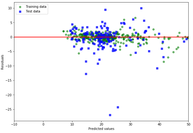
# 残差プロット
# %matplotlib inline
plt.figure(figsize = (10, 7))
plt.scatter(y_train_pred, y_train_pred - y_train, c = 'green', marker = 'o', s = 35, alpha = 0.5, label = 'Training data')
plt.scatter(y_test_pred, y_test_pred - y_test, c = 'blue', marker = 's', s = 35, alpha = 0.7, label = 'Test data')
plt.xlabel('Predicted values')
plt.ylabel('Residuals')
plt.legend(loc = 'upper left')
plt.hlines(y = 0, xmin = -10, xmax = 50, lw = 2, color = 'red')
plt.xlim([-10, 50])
plt.show()

横軸に予測値（または説明変数）をとり、縦軸に回帰残差をとってプロットした残差プロットを見てみましょう。
残差プロットを見ると、検証用のデータより学習データにより適合したモデルであることがわかります。

今回作成したプログラム

分類のプログラム

import csv
import numpy as np

with open('./titanic.csv','r') as csvfile:
    titanic_reader = csv.reader(csvfile,delimiter=',',quotechar='"')

    #特徴量の名前が書かれたHeaderを読み取る
    row = next(titanic_reader)
    feature_names = np.array(row)

    #データと正解ラベルを読み取る
    titanic_x, titanic_y = [],[]
    for row in titanic_reader:
        titanic_x.append(row)
        titanic_y.append(row[2]) #正解ラベルは3列目の"survived"

    titanic_x = np.array(titanic_x) #型をリストからnumpy.ndarrayにする
    titanic_y = np.array(titanic_y) #型をリストからnumpy.ndarrayにする

print(feature_names)
print(titanic_x[0],titanic_y[0])


# class(1),age(4),sex(10)を残す
titanic_x = titanic_x[:,[1, 4, 10]]
feature_names = feature_names[[1, 4, 10]]

print(feature_names)
print(titanic_x[12],titanic_y[12])


# 年齢の欠損値を平均値で埋める
ages = titanic_x[:,1]
# NA以外のageの平均値を計算する
mean_age = np.mean(titanic_x[ages != 'NA',1].astype(float))

# 上記コードでValueError: could not convert string to float:というエラーが出る場合は、下記のように変更してください。
# mean_age = np.mean(titanic_x[ages != '',1].astype(float))

# ageがNAのものを平均値に置き換える
titanic_x[titanic_x[:, 1] == 'NA',1] =mean_age


from sklearn.preprocessing import LabelEncoder
enc = LabelEncoder()
label_encoder = enc.fit(titanic_x[:, 2])
print('Cateorical classes:',label_encoder.classes_)

integer_classes = label_encoder.transform(label_encoder.classes_)
print('Integer classes:',integer_classes)

t = label_encoder.transform(titanic_x[:, 2])
titanic_x[:,2] = t

print(feature_names)
print(titanic_x[12],titanic_y[12])


from sklearn.preprocessing import OneHotEncoder
enc = LabelEncoder()
label_encoder = enc.fit(titanic_x [:, 0])
print("Categorical classes:", label_encoder.classes_)
integer_classes = label_encoder.transform(label_encoder.classes_).reshape(3, 1)
print("Integer classes:", integer_classes)
enc = OneHotEncoder()
one_hot_encoder = enc.fit(integer_classes)

# 最初に、Label Encoderを使ってpclassを0-2に直す
num_of_rows = titanic_x.shape[0]
t = label_encoder.transform(titanic_x[:, 0]).reshape(num_of_rows, 1)
#次に、OneHotEncoderを使ってデータを1, 0に変換
new_features = one_hot_encoder.transform(t)
#1,0になおしてデータを統合する
titanic_x = np.concatenate([titanic_x, new_features.toarray()], axis = 1)
#OnehotEncoderをする前のpclassのデータを削除する
titanic_x = np.delete(titanic_x, [0], 1)
#特徴量の名前を更新する
feature_names = ['age', 'sex', 'first class', 'second class', 'third class']

# Convert to numerical values
titanic_x = titanic_x.astype (float)
titanic_y = titanic_y.astype (float)

print(feature_names)
print(titanic_x[0],titanic_y[0])

from sklearn.model_selection import train_test_split
x_train, x_test, y_train, y_test = train_test_split(titanic_x, titanic_y, test_size=0.25, random_state=0)


from sklearn import metrics
def measure_performance(x,y,clf, show_accuracy=True,show_classification_report=True, show_confussion_matrix=True):
    y_pred=clf.predict(x)
    if show_accuracy:
        print("Accuracy:{0:.3f}".format(metrics.accuracy_score(y, y_pred)), "\n")

    if show_classification_report:
        print("Classification report")
        print(metrics.classification_report(y, y_pred), "\n")

    if show_confussion_matrix:
        print("Confussion matrix")
        print(metrics.confusion_matrix(y, y_pred),"\n")

from sklearn import tree
clf = tree.DecisionTreeClassifier(criterion='entropy', max_depth= 3, min_samples_leaf = 5)
clf = clf.fit(x_train, y_train)

import pydotplus
from sklearn.externals.six import StringIO
dot_data = StringIO()
tree.export_graphviz(clf, out_file=dot_data,feature_names = ['age','Sex','1st_c1ass','2nd_class','3rd_class'])
graph = pydotplus.graph_from_dot_data(dot_data.getvalue())
graph.write_pdf("tree.pdf")

#決定木モデルの評価
measure_performance(x_train, y_train, clf)


from sklearn.ensemble import RandomForestClassifier
clf = RandomForestClassifier(n_estimators=30, random_state=0)
clf = clf.fit(x_train, y_train)

#ランダムフォレストモデルの評価
measure_performance(x_train, y_train, clf)

回帰のプログラム

# ======= 回帰 =======
# 必要なライブラリのインポート
import numpy as np
import pandas as pd
import matplotlib.pyplot as plt
from pandas import DataFrame
from sklearn.datasets import load_boston
from sklearn.model_selection import train_test_split
from sklearn.ensemble import RandomForestRegressor

# データの読み込み
boston = load_boston()
df = DataFrame(boston.data, columns = boston.feature_names)
df['MEDV'] = np.array(boston.target)

# 説明変数及び目的変数
X = df.iloc[:, :-1].values
y = df.loc[:, 'MEDV'].values

# 学習用、検証用データに分割
(X_train, X_test, y_train, y_test) = train_test_split(X, y, test_size = 0.3, random_state = 0)

# モデル構築
forest = RandomForestRegressor()
forest.fit(X_train, y_train)

# 予測値を計算
y_train_pred = forest.predict(X_train)
y_test_pred = forest.predict(X_test)

# MSEの計算
from sklearn.metrics import mean_squared_error
print('MSE train : %.3f, test : %.3f' % (mean_squared_error(y_train, y_train_pred), mean_squared_error(y_test, y_test_pred)) )

# R^2の計算
from sklearn.metrics import r2_score
print('MSE train : %.3f, test : %.3f' % (r2_score(y_train, y_train_pred), r2_score(y_test, y_test_pred)) )

# 残差プロット
# %matplotlib inline
plt.figure(figsize = (10, 7))
plt.scatter(y_train_pred, y_train_pred - y_train, c = 'green', marker = 'o', s = 35, alpha = 0.5, label = 'Training data')
plt.scatter(y_test_pred, y_test_pred - y_test, c = 'blue', marker = 's', s = 35, alpha = 0.7, label = 'Test data')
plt.xlabel('Predicted values')
plt.ylabel('Residuals')
plt.legend(loc = 'upper left')
plt.hlines(y = 0, xmin = -10, xmax = 50, lw = 2, color = 'red')
plt.xlim([-10, 50])
plt.show()

まとめ

この記事ではランダムフォレストを学習しました。
ランダムフォレストは、アンサンブル学習の一種で複数の決定木を用いて学習します。
アルゴリズムとしての特徴を抑えて、他のアルゴリズムと使い分けられるようにしましょう。

Pythonや機械学習を効率よく学ぶには？

Pythonや機械学習を効率よく学ぶには、普段からPythonを利用している現役のデータサイエンティストや機械学習エンジニアに質問できる環境で学ぶことです。
質問し放題かつ、体系的に学べる動画コンテンツでデータ分析技術を学びたい方は、オンラインで好きな時間に勉強できるAI Academy Bootcampがオススメです。受講料も業界最安値の35,000円（６ヶ月間質問し放題＋オリジナルの動画コンテンツ、テキストコンテンツの利用可能）なので、是非ご活用ください。